This is an old revision of the document!
Calculator of inductance of a straight coaxial cable
* This page is being edited and may be incomplete or incorrect.
| | Stan Zurek, Calculator of inductance of a straight coaxial cable, Encyclopedia Magnetica, https://www.e-magnetica.pl/doku.php/calculator/inductance_of_coaxial_cable, {accessed: 2025-03-13} |
| |
|
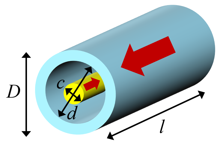
Inductance of a straight coaxial cable with round (circular) cross-section (with return current path) can be calculated withe the equation as specified below.
Equations
Note: Several assumptions are made for these equations: 1) The return path is considered so this equation represents a “closed-loop” electrical circuit. 2) The length of the wire is assumed to be significantly longer than its diameter(s) (c,d,D « l), otherwise the calculation errors might be excessive. 3) All the materials and the surrounding medium are assumed to be non-magnetic (μr = 1). 4) The current is uniformly distributed inside the wire (no skin effect) for the DC case. 5) The equations were converted here to be consistent with SI units.
| Inductance of a straight round magnetic wire or conductor | ||
|---|---|---|
| Sources: [1] Frederick W. Grover, Inductance Calculations: Working Formulas and Tables, ISA, New York, 1982, ISBN 0876645570 and [2] Clayton R. Paul. Inductance: Loop and Partial, Wiley-IEEE Press, 2009, New Jersey, ISBN 9780470461884 [3] Edward B. Rosa, The self and mutual inductance of linear conductors, Department of Commerce and Labor, Bulletin of the Bureau of Standards, Volume 4, 1907-8, Washington, 1908, {accessed 2025-01-06} |
||
| (1) [1] Grover, eq. (232), p. 280 (assumes infinitely thin shield) | $$ L_{AC} = \frac{μ_0 ⋅ l}{2⋅π} ⋅ \left( ln \left( \frac{d}{c} \right) + \frac{T(x)}{4} \right) $$ | (H) |
| (2) [1] Grover, eq. (24), p. 42 (original, with the discrepancy) | $$ L = \frac{μ_0 ⋅ l}{2⋅π}⋅\left( ln \left( \frac{D}{c} \right) + \frac{2· \left( \frac{d}{D} \right) ^2}{1-\left( \frac{d}{D} \right) ^2} ⋅ ln \left( \frac{D}{d} \right) - \frac{3}{4} + ξ_Z \right) $$ | (H) |
| (3) [1] Grover, eq. (24), p. 42 (see the note below about the possible discrepancy) | $$ L = \frac{μ_0 ⋅ l}{2⋅π}⋅\left( ln \left( \frac{d}{c} \right) + \frac{2· \left( \frac{d}{D} \right) ^2}{1-\left( \frac{d}{D} \right) ^2} ⋅ ln \left( \frac{D}{d} \right) - \frac{3}{4} + ξ_Z \right) $$ | (H) |
| (4) [2] Paul, eq. (4.29), p. 132 [3] Rosa, eq. (58), p. 333 (for high frequency limit) | $$ L = \frac{μ_0 ⋅ l}{2⋅π}⋅ln \left( \frac{d}{c} \right) $$ | (H) |
| where: $μ_0$ - magnetic permeability of vacuum (H/m), $l$ - wire length (m), $D$ - outer diameter (m) of the shield conductor, $d$ - inner diameter (m) of the shield conductor, $c$ - outer diameter (m) of the solid inner conductor, $ξ_Z$ - Grover's function from Table 4 (unitless) approximated here by S. Zurek with a polynomial function, for ratio $z = d/D$ (unitless): | ||
| (1.1) Grover's Table 4 with Zurek's approximation by polynomials | $$ ξ_Z = 0.1705⋅z^3 - 0.3979⋅z^2 - 0.0214⋅z + 0.25 $$ | (unitless) |
| The original Grover's equation appears to be incorrect, with the first logarithm given as $ln(D/c)$ but it is clear from Grover's description that it should be $ln(d/c)$, as this is the limit for high frequency, and as listed for example by Paul [2]. Grover's and Paul's equations are based on radii, but all variables are used as ratios, so diameters can be used directly instead because ratio of radii is equal to the ratio of the corresponding diameters. | ||
| → → → Helpful page? Support us! → → → | PayPal | ← ← ← Help us with just $0.10 per month? Come on…  ← ← ← |