Magnetic field - a region in space, in which magnetic forces are observable. Magnetic forces are mechanical forces acting as a result of magnetic interactions.

Magnetic field B acting with a magnetic force F_m on a positive electric charge q moving with velocity v, direction of F_m is perpendicular to both B and v

^{S. Zurek, E-Magnetica.pl, CC-BY-4.0}

Magnetic field is always generated around electric current, or more generally by moving electric charges or by varying electric field E, as well as intrinsic magnetic dipole moments of sub-atomic particles.¹⁾²⁾³⁾ The existence of magnetic field is responsible for magnetism and electromagnetism.

In vacuum, a force F (Lorentz force) acting on an electric charge q moving with velocity v is due to the electric field E and magnetic field B (magnetic flux density): $\vec{F} = q·\vec{E} + q·\vec{v} × \vec{B}$

The field which satisfies the action of the B vector in the Lorentz force equation is assumed to be the definition of magnetic field.⁴⁾⁵⁾

In physics, a field is a quantity or value assigned to each point in space or volume. Therefore, magnetic field can be mathematically described by assigning physical quantity to each point in space filled with such field. Depending on the required mathematical treatment the description can be a scalar field of vector field, also being a function of position or time.⁶⁾

In order to fully quantify the effects of magnetic field in a given material or medium, it is practical to use two quantities such as magnetic flux density B and magnetic field strength H.

Both B and H are strictly defined in terms of measurement units as well as their physical and technical meaning.⁷⁾⁸⁾⁹⁾ However, there are two main approaches to the analysis, usefulness and importance of B and H magnetic fields: theoretical physics and engineering.

If the same system of units is used, e.g. SI, then both approaches are exactly equivalent, in terms of the numerical values and units. Only the names or problematic, not the units or mathematical calculations.¹⁰⁾

These two approaches are complementary, giving access to a type of equation which is more useful for a given calculation. One is not “better” than the other, simply because it is considered more “fundamental” by one group of people. The “quality” of either form of definition is only as good as its usefulness for a specific purpose, such as calculation of effects with relativistic phenomena, or designing an efficient transformer or electromagnet.

However, theoretical physics puts more emphasis on B, whereas in engineering both H and B are treated as equally important. Naming conventions can differ significantly. Additionally, the previously used CGS system of units (still used by some countries and branches of science) has yet another set of names and coefficients. All this creates an often confusing mix, with many books on electromagnetisms giving full list of conversion factors between the different systems.

See also: Confusion between B and H.

In particular attention has to be paid to some equations, because they might be written in a given form which requires certain implicit conditions to be met - these conditions are often not stated.

For instance, the Biot-Savart law written in the physics form $B = f (μ_0 · I)$ is valid only in vacuum, whereas the engineering form $H = f (I)$ is more general, and valid for any uniform isotropic medium.

In the theoretical approach more emphasis is put on the derivation of equations from first principles, and usefulness of a given expressions for deriving other equations. Microscopic (atomic and sub-atomic level) understanding is fundamental, but between and inside the atoms of any matter there is vacuum. Ferromagnetic materials receive limited attention or not at all¹¹⁾, with the explanations following those of the engineering approach.¹²⁾¹³⁾

The units are used observing all the usual physical and mathematical rules. However, the relationship between the units and the names of the variables appear to be treated less rigorously, with tesla and A/m used almost interchangeably, for B, H and M, using the magnetic constant $μ_0$ as a conversion tool.

From theoretical physics viewpoint, the only form of magnetic field required for all analysis is the magnetic field B, which is regarded as “indisputably fundamental”.¹⁴⁾¹⁵⁾ The definition of B is a field which causes the force described by equation (1).

Depending on type of notation in various literature, either the notation with bold fonts denoting vectors (equation (1a)) or with the arrows above the variables (equation (1b)) can be used - both are precisely equivalent.

Force due to electric field acts in the direction of that field (dot product “·” in equations (1ab)). Force due to magnetic field acts perpendicularly to both the direction of movement of the charge and the direction of magnetic field (cross product “×” in equations (1ab)).

Lorentz force acting on a positive charged particle q: a) force F_e in electric field E, b) force F_m in magnetic field B, c) total force F = F_e + F_m in both fields; green solid arrow shows velocity and direction of movement, green dotted arrow how the trajectory develops

^{S. Zurek, E-Magnetica.pl, CC-BY-4.0}

Other names for B such as “magnetic flux density” and “magnetic induction” are even regarded as “absurd choice”.¹⁶⁾ The quantity H is treated as “auxiliary” and having “no name”.¹⁷⁾¹⁸⁾ Some theoreticians even regard the SI units as “arbitrary and a little daft”.¹⁹⁾ Other systems of units can be used for theoretical calculations, such as Lorentz-Heaviside or natural units, which can be defined with permeability of vacuum or speed of light as unity (unitless), which can simplify certain calculations.²⁰⁾

Magnetic field B is generated by electric current and intrinsic magnetic dipole moments of subatomic particles.

Magnetic force, as defined by the Lorentz force is proportional to B, and such force is taken as the definition of flux density B. The full form of Maxwell's equation always shows B, not H. This is because the divergence of B is always zero, whereas it can be non-zero for H.²¹⁾

On a microscopic level, between and inside the atoms, there is vacuum and B can be used for all the calculations.

If SI units are used then B has the dimension of tesla.

Magnetic properties of matter are a consequence of macroscopic averaging of microscopic effects, especially due to vector summation of magnetic dipole moments of subatomic particles (and atoms), which can align to the magnetic field applied to the material. The material responds with magnetisation M when exposed to some magnetic field B. If complete alignment of all free magnetic moments is achieved then the material is said to be magnetically saturated, and value of M cannot increase any more.²²⁾

Magnetisation M is the sum of magnetic dipole moments per unit of volume V

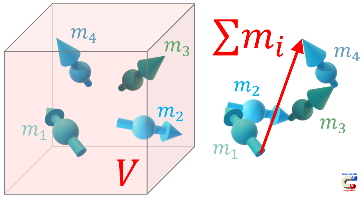
^{S. Zurek, E-Magnetica.pl, CC-BY-4.0}

Magnetisation M is defined²³⁾²⁴⁾ as the sum of magnetic moments per unit volume, within a given material, as per equation (2).

In many physics research papers the magnetisation is expressed as mass magnetisation, with the response measured by a unit of mass, rather than a unit of volume, with the popular unit of emu/g.^25)26)27)

The conversion factor to SI units is: 1 emu/g = 1 A⋅m²/kg, and density of the material can be used to convert it to volume magnetisation.²⁸⁾

Magnetisation M (A/m) is sometimes also called “magnetic polarisation”.²⁹⁾³⁰⁾

In research papers written by theoretical physicist, if magnetisation M is used to express a quantity in measurable in the units of tesla (rather than A/m), then the value is simply multiplied by $μ_0$ (permeability of vacuum) or stated directly in teslas (with an implicit assumption that it is multiplied by $μ_0$).³¹⁾

Even in some excellent books on theoretical electromagnetism (e.g. references ³²⁾³³⁾) the polarisation J is not mentioned (and hence not defined).

However, magnetic polarisation J can be defined and calculated as: $J = μ_0 · M$, with the unit of tesla.³⁴⁾

From a macroscopic viewpoint, there are additional effects because atoms interact with each other magnetically, and it is recognised that an “auxiliary” field H can be defined, and although “illogical” it can be “useful”, because it can be directly related to free currents, such that a direct relationship between the current and H can be stated.³⁵⁾

Therefore, the auxiliary field H is defined³⁶⁾³⁷⁾ as in equation (3).

Even if SI units are used, sometimes H is expressed in teslas.³⁸⁾³⁹⁾

Magnetic susceptibility χ can be defined in more than one way.⁴⁰⁾ For materials which respond linearly to the applied magnetic field, with the assumption that M is proportional to B or the H, volume susceptibility can be defined as:⁴¹⁾

For diamagnets susceptibility is negative, for paramagnets it is positive. For vacuum it is zero.

These two definitions (4a, 4b) differ so that:

For non-magnetic materials $χ << 1$ and the difference in negligible,⁴²⁾ and $χ = χ_{(H)} \approx χ_{(B)}$.

However, for large values of $χ$, as encountered in ferromagnets, the definitions (4a,b) are less useful, because (5) diverges, and permeability is used instead of susceptibility.

Magnetic permeability μ is defined in relation to susceptibility:

and can be used as the proportionality factor between B and H:

However, there are limitations with this equation, because in ferromagnets $μ_r$ is a non-linear function of B or H.

In the engineering approach, less emphasis is put on the fundamental physical concepts, and more on the properties directly measurable quantities, useful for practical applications and design of devices. Magnetic quantities are linked to the macroscopic electrical quantities which can be directly measured or controlled in electromagnetic devices, such as electric voltage and current.

This leads to a different concept of excitation-response relationship and the naming convention, as defined by the international SI system of units.⁴³⁾

See also the main article: Magnetic field strength.

Magnetic field strength H is measured in amperes per metre, A/m (or scaled by the SI multipliers: kA/m, MA/m, etc.)

Biot-Savart law: $P$ - point at which the magnetic field strength $\vec H$ is calculated, $R$ - perpendicular distance from conductor, $I$ - current, $\vec J$ - current density, $d \vec l$ - infinitesimal length of conductor contributing to magnetic field, $r$ - distance, $\vec r$ - path vector, $\hat r$ - unit vector along direction of $r$, $\theta$ - angle between $d \vec l$ and $r$

^{S. Zurek, E-Magnetica.pl, CC-BY-4.0}

Electric currents are the source of H. The proportionality is defined by the length of path under consideration (magnetic path length), and the total amount of current I, contained in a single conductor, or a number N of conductors. The calculation of H can be based either on the Biot-Savart law or on Ampere's circuital law, with both approaches giving identical results for the same configuration.⁴⁴⁾⁴⁵⁾

From Biot-Savart law:⁴⁶⁾

In an alternative approach, an integral over a closed path of the tangential component of H gives the value of the enclosed free current.⁴⁷⁾ From Ampere's circuital law:

Electric current I generates around itself magnetic field strength H

^{S. Zurek, E-Magnetica.pl, CC-BY-4.0}

As shown above, both equations can be formulated so that the magnetic permeability does not appear - magnetic properties of matter (or permeability of vacuum) are not relevant for generation of H (strictly applicable only in a uniform and isotropic medium, regardless if it is non-magnetic, magnetic, non-linear, etc.)⁴⁸⁾

Equation (9) can be rearranged so that the electric current I produces around itself well-defined magnetic field strength H, whose amplitude is independent of the type of magnetised material. For a uniform medium (no additional sources of magnetic field, such as magnetic poles due to demagnetising factor) there is a direct proportionality between I and H (e.g. instantaneous change of I produces instantaneous change of H, assuming changes negligibly slow with the speed of light):

For example, a current of 1 A in a straight wire, produces H circulating around the wire (according to the right-hand rule), such that at a radius of r = 0.1 m (from the centre of the wire), related to the circle with path length $l = 2·π·r$ = 0.628 m, which is equal to around H = 1.59 A/m (see also: Calculator of magnetic field of straight round conductor).

Simple magnetic circuit: core and air gap

^{S. Zurek, E-Magnetica.pl, CC-BY-4.0}

If the medium is not isotropic, or there are several different materials then the field distribution is affected by demagnetising field caused by magnetic poles. These poles become new sources of magnetic field which change distribution of the original applied field.⁴⁹⁾

The product N·I is also known as magnetomotive force (MMF), which can be thought of as the applied excitation, and the component H·l represents the drop of MMF in a magnetic circuit (as an analogy to voltage drop in an electric circuit). If the magnetic circuit comprises a high-permeability magnetic core and an air gap (both of uniform cross-sectional area) then equation (10) can be applied as:

and it is widely used for design of electric motors, electromagnets, magnetic sensors, flyback transformers, etc.

In CGS units H is measured in oersteds (Oe), with the conversion factor: 1 Oe = 1000 / (4⋅π) A/m ≈ 79.58 A/m.⁵⁰⁾

See also the main article: Magnetic flux density.

In ferromagnets the B-H relationship is non-linear, history-dependent and typically anisotropic

^{S. Zurek, E-Magnetica.pl, CC-BY-4.0}

Magnetic flux density B is a response of a medium when magnetised with H.⁵¹⁾ The amplitude of B depends both on the applied excitation as well as the material properties (and the magnetic history of the material, in case of prior magnetisation of ferromagnets).

As mentioned above, H can be quantified with respect to the magnetising current (but direct measurement methods are also used, such as H-coil). B is measured by using the Faraday's law of induction (one of the Maxwell's equations), which can be written as:⁵²⁾⁵³⁾

Illustration of relationship in a ferromagnet between magnetic field strength H, magnetic flux density B, magnetisation M, and magnetic polarisation J

^{S. Zurek, E-Magnetica.pl, CC-BY-4.0}

Therefore, the value of B (or a continuous waveform) can be derived calculating an integral of the measured voltage (by an analogue circuit with an integrating opamp, or by digital calculations of a sampled signal).

The difference of sign in both equations arises, because (12a) describes electromotive force (EMF) induced internally in the given sensing coil (B-coil), but this information is not available in any way - only the external voltage (12b) can be measured. This difference is often implicitly assumed, but sometimes even misunderstood, showing the minus sign even for measured voltages.⁵⁴⁾

Because equation (12a,b) defines the relationship by means of a derivative, it is not possible to measure a DC component in an as easy was as the AC component. Some variability is required, which can be achieved by moving the coil (ballistic measurement, vibrating coil magnetometer) or moving the sample (vibrating sample magnetometer).

For energy transformation it is very useful to utilise the AC excitation. If a full cycle of excitation is applied, and both waveforms of H and B are measured then a B-H loop (hysteresis loop) can be plotted, as shown in the image.

The area of the loop is proportional to all the energy lost during magnetisation of a material, and it is a fundamental tool by which total magnetic losses are measured in a material. All components of magnetic loss are automatically included (hysteresis, eddy currents, excess loss) which is why it is so important practically to accurately measure both: the magnetic field strength H and the magnetic flux density B. Equation (12c) is the basis for design of all power transformers operating with sinusoidal voltage.⁵⁵⁾

There are several internation standards defining such loss measurement procedures for the industrially important soft magnetic materials, such as electrical steels.⁵⁶⁾⁵⁷⁾

See also the main article: Magnetic permeability.

Permeabilities of magnetic materials (e.g. ferromagnets $μ_{ferro}$) are much higher than non-magnetic materials (e.g. vacuum $μ_0 = μ_{vac}$, diamagnets $μ_{dia}$ and paramagnets $μ_{para}$)

^{S. Zurek, E-Magnetica.pl, CC-BY-4.0}

Magnetic permeability μ is the quantity expressing the proportionality factor between H and B. Soft magnetic materials are pivotal to efficient energy transformation, so they receive a lot of attention, and the permeability value is used as a figure of merit. For any such material it can be written that:

For vacuum, the B-H relationship is fully linear, and $μ_0$ = 4·π·10^-7 (H/m) which is a universal physical constant,⁵⁸⁾ and $μ_r = 1$. In practice, for most non-magnetic materials $μ_r$ is so close to unity that the difference is neglected.⁵⁹⁾

Permeability of a medium different than vacuum can be defined as a product of dimensionless number relative to $μ_0$. Hence, $μ = μ_r · μ_0$. So for instance, relative permeability $μ_r$ = 100 means that the given material has permeability 100 times higher than the value of $μ_0$ (as measured in H/m). This means that for the same applied H the material will respond with B that is 100 times greater than it would be for vacuum (or non-magnetic material).

Ratio B / H at a given point of magnetisation curve can be used for calculating permeability value

^{S. Zurek, E-Magnetica.pl, CC-BY-4.0}

For uniform and isotropic materials permeability can be expressed as scalar, even though H and B are vectors. For anisotropic materials permeability is different in various directions and vector or tensor approach has to be used for more correct representation. However, in practice the scalar approach is often used because of its simplicity (and sufficiently accurate results for most practical purposes, such as design of magnetic circuits).

When excitation H varies in time then additional effects are introduced, like for instance eddy currents, which affect the apparent permeability. The effective permeability is also affected by shape anisotropy. In magnetic material like ferromagnets the relationship between B and H can be non-linear, history-dependent and highly anisotropic.

There are many different types of permeability which can be derived from measured B-H characteristics, as needed for a specific practical application: relative, amplitude, reversal, impulse, etc. The calculation is always performed as a ratio $μ = f (ΔB/ΔH)$, with the delta Δ defining the reference point (e.g. origin of the graph, position of the previous impulse, etc.)

Soft magnetic materials saturate if sufficiently high excitation is applied. This causes the ratio of B/H and hence also the permeability to reduce. When approaching to full saturation relative permeability will approach unity (i.e. the same as for vacuum).

For hard magnetic materials the value of permeability is of little use, and it is not discussed with the same depth, or even omitted in some books.⁶⁰⁾

Susceptibility is rarely used in engineering applications.

Electric charges (in the form of electrons and protons) are the most basic components responsible for all macroscopic electrical phenomena. However, it is far more useful in practical electrical engineering to operate with such values as voltage $V$ (related to concentration and distribution of electric charges) and electric current $I$ (representing movement of electric charges).

Combination of these two values fully quantifies the effects of electricity, such as dissipated power P, because $P = V·I$. Additional parameters such as resistance R define proportionality of electrical response or V-I relationship (Ohm's law) $I = V / R$ for a given material. Conductance G (reciprocal of resistance, $G = 1 / R$) can be used to express the equation in a different, but equivalent form: $I = G·V$.

By analogy, in engineering, both magnetic flux density $B$ and magnetic field strength $H$ (or their equivalents) are required for quantifying the effects of magnetism in matter, for example stored or lost energy.⁶¹⁾ These two quantities are defined separately in the International System of Units (SI), with $H$ having the unit of ampere per metre (A/m), and $B$ the unit of tesla (T). ⁶²⁾⁶³⁾

Energy density in a given magnetic material can be calculated as $E_{density}=B·H$. Permeability μ defines the proportionality of a magnetic response: $B = μ·H$. These relations are widely used in the engineering approach.

Magnetic field is a concept of energy contained in a given volume of space. This energy can be physically and mathematically described by various means or quantities. There are six most frequently used magnetic quantities, which are interrelated, as shown in the table below.

Magnetic field contains energy whose density per volume can be calculated with the following equation (for a medium with a constant permeability).⁶⁴⁾

The energy and power dissipated in a magnetically soft material can be calculated by integrating over a full cycle of AC excitation:⁶⁵⁾

The temporary energy storing capability can be utilised with a non-magnetic material, e.g. in the air gap of a choke or a flyback transformer. In such a magnetic circuit, if $B_{material} \approx B_{gap}$ (which is typically the case for a small air gap) then the value of $H$ will differ by the factor of a relative permeability of of the material, so the air gap can store significantly more energy than the magnetic core.

Optimum operating point P for a permanent magnet is where the product B and H reaches maximum BH_max⁶⁶⁾

^{S. Zurek, E-Magnetica.pl, CC-BY-4.0}

In permanent magnets, the theoretical maximum amount of energy density which can be obtained for a given material is proportional to the square of the remanence value of $B_r = J_r$. In practice only around 60% of this value is achievable.⁶⁷⁾

The optimum operating point P for a permanent magnet is where the product B and H reaches a maximum BH_max.⁶⁸⁾⁶⁹⁾

It is difficult to give a simple definition of magnetic or electromagnetic field.

Progress of science and technology is based on some quantities which so far cannot be defined precisely. For example, the fundamental electric charge q or time t are referred to without defining what they are. Scientists can describe, but still cannot explain what exactly is time or electric charge. The assumption is that they exist, have some physical meaning and are measurable within the given system of units.⁷⁰⁾

Magnetic field can be produced by electric current, which itself is defined as the flow of electric charge in time. It is empirically known that magnetic field acts with mechanical force on moving charged particles in specific ways described by Maxwell's equations. Therefore, the acting of such specific mechanical forces ultimately defines the presence or absence of magnetic field.

Or in other words, the detection of magnetic field can be reduced to analysis of such mechanical forces acting on moving electrically charged particles. This is the reason for the opening definition in this article which refers only to magnetic forces (mechanical forces caused by magnetic field). Such definition seems somewhat circular, but as stated above due to the insofar inexplicable nature of underlying physics it cannot be made more precise.

For these reasons many books and publications on magnetism either do not give definition at all or use similar definition as given above in this article. Typical examples are quoted in the table below.

The name electromagnetic field is used to refer to a field continuously variable in time. It is said that variable electric field (moving electric charges) produces variable magnetic field, and in turn, variable magnetic field produces variable electric field. This result in electromagnetic field, in which the electric and magnetic components are inseparably interlinked.⁷⁷⁾

However, if for instance the magnetic field is generated by a permanent magnet then the resulting field does not vary with time so the electric field component is not generated. Such field is then referred to as magnetostatic field (constant in time) in order to explicitly distinguish it from “electromagnetic field” (which is variable in time and coexists with the variable electric field component).

The distinction is similar as in analysis of electrical circuits with electrostatic effects.⁷⁸⁾ If there are no changes of charge distribution (i.e. there are no currents flowing) then the analysis is said to be electrostatic, to distinguish it from other cases.

Magnetic field around a moving electron; the distribution of magnetic field can be calculated from Biot-Savart law assuming that the velocity if much smaller than speed of light⁷⁹⁾

^{S. Zurek, E-Magnetica.pl, CC-BY-4.0}

In its narrow meaning, the name “magnetic field” refers only to the magnetostatic field or the magnetic component of the electromagnetic field.

However, in a wider sense “magnetic field” is also used to refer to electromagnetic field. This is because electromagnetic field contains the magnetic field component in which the magnetic forces are “observable” as per definition of magnetic field (see also the table above, with the quotes of various definitions). The narrower or wider meaning is typically clear from the context, if not explicitly defined.

A moving electric charge has attached to it a magnetic field, whose distribution follows the Biot-Savart law. Such magnetic is called velocity field and does not radiate away if the charge moves at a constant velocity. Electrostatic field extends away to infinity, from either static or moving charge.

However, when the charge gets accelerated (or decelerated), for the whole duration of acceleration, both the electric and magnetic field surrounding the charge gets distorted. The ripple comprises both components of field, and radiates away from the charge, carrying with it some energy.

Diagram illustrating generation of electromagnetic field by an electric charge: a static charge (grey small circle at the centre) generates electrostatic field (blue area) which statically extends away into space. A sudden acceleration of the charge (dark blue small circle) creates an electromagnetic pulse (red ring) which radiates away into space at the speed of light, and the space far away still contains the electrostatic field from the time when the charge was stationary (as indicated by grey lines). A charge moving at a constant velocity v generates electric and magnetic field attached with the charge (green area). The field lines (black lines) show the direction and intensity of electric field.⁸⁰⁾

^{S. Zurek, E-Magnetica.pl, CC-BY-4.0}

If the charge is moved in a sinusoidal manner then the radiation also takes a sinusoidal character, providing a basis for wireless transmission of information (equivalent to some amount of energy) through the volume of space.

Reception of electromagnetic waves is the same process but in reverse - the electric and magnetic components of the field can move the charges in the antenna, and thus produce voltage and current, which can be then processed by an appropriate electronic circuitry, to recover the information (wireless communication) or energy (wireless charging). Resonating LC circuits are used to improve efficiency of transmission-reception.

The concepts of near field and far field are introduced in analysis of electromagnetic fields. All magnetostatic effects can be treated as occurring in the near field region.⁸¹⁾

Electromagnetic wave with wavelength λ, propagating in direction x, comprising the component of electric field E in phase with the magnetic field B; all three directions (E, B and x are orthogonal to each other⁸²⁾

^{S. Zurek, E-Magnetica.pl, CC-BY-4.0}

Static magnetic field penetrates matter, with the exception of superconductors which can expel the field from their inside (B=0, H>0, M<0), by sustaining surface currents.⁸³⁾

Mathematical equations can be used to describe electromagnetic field either as a wave (electromagnetic waves) or as particles (e.g. photons), and both representations were proved to be correct from a specific experimental point of view. If electromagnetic field is a wave then it is unknown in what medium such wave should exist, because it propagates equally well through vacuum, which does not contain any matter.

In quantum field theories such as quantum chromodynamics (QCD) the absence of elementary particles does not necessarily have to mean the lack of any medium. For instance, it is possible to analyse the effect of electromagnetic field on the vacuum in various energy regimes. As a result of such analysis the vacuum is no longer “free space” and theoretically particles can be continuously created and annihilated.⁸⁴⁾ Such property can be therefore responsible for allowing the electromagnetic energy to propagate in a seemingly “empty” medium.

In quantum field theory, electrostatic forces between two charges can be thought of as arising due to exchange of virtual photons, which are “fluctuations” of empty space.⁸⁵⁾

See also the main article: Magnetic field lines.

Magnetic field lines are a theoretical concept and there are no “lines” in reality. However, this concept is very useful in visualising the distribution of magnetic flux or electric field. The lines represent direction which is tangent to the direction of the given vector quantity, such as magnetic flux density at a given location.

If iron particles are placed in the vicinity of a magnet then they will form elongated structures which follow such lines extending between the magnetic poles. In a similar way, a magnetic compass placed next to a magnet or electromagnet will have its needle following the contours created by magnetic particles.

FEM simulation illustrating imaginary magnetic field lines around a bar magnet

^{S. Zurek, E-Magnetica.pl, CC-BY-4.0}

Iron filings create elongated line-like structures around a permanent magnet

^{S. Zurek, E-Magnetica.pl, CC-BY-4.0}

“Magnetic field lines” around an electromagnet, as indicated by small compasses

^{S. Zurek, E-Magnetica.pl, CC-BY-4.0}

“Magnetic field lines” extend into 3D space around a magnet ^{by JanDerChemiker, CC-BY-3.0}

For this reason they can be also called “magnetic force lines” and can be used to visualise the magnetic field around a given source, when plotted on a given cross-section (two-dimensional plane). The density of the lines (e.g. number of lines per unit area) represents the amplitude (more lines closer to each other means greater amplitude). The lines can never cross and each line is a closed curve (i.e. has no beginning or end). The lines are a theoretical concept and thus can extend over infinite lengths.

From purely theoretical view point the magnetic field lines can extend to infinity, which would imply that a single moving electron could produce magnetic field extending over the whole universe - and if electromagnetic radiation takes place the electromagnetic field can indeed propagate vast distances, throughout the universe.

However, the intensity of magnetic field reduces with the distance from the source. Therefore, in practice the fields become vanishingly small at sufficiently long distances from the given source.⁸⁶⁾

Similar concept is used for electric field lines, but they start at positive charges and end at negative ones (electric field lines have sources, magnetic field lines do not).

Magnetic dipole moment $\vec m$ of a loop of current $\vec I$ with the loop area $A$ and unit vector $\vec a$ (normal to $A$)

^{S. Zurek, E-Magnetica.pl, CC-BY-4.0}

A circular loop with current is one of the simplest circuits which generates magnetic field. At large distance from such loop the field is similar to the field produced by a magnetic dipole of two hypothetical magnetic monopoles with opposing charges separated by a given distance (per analogy to a dipole created by two electric charges).

Magnetic moment will act on a magnetic dipole placed in an external magnetic field. The acting torque will be proportional to the cross product of the two vectors: magnetic moment and flux density.⁸⁷⁾

Magnetic moments are important in analysis of magnetic phenomena, because an electron orbit in an atom is in some sense analogous to a loop of current - hence having a magnetic moment associated with it. This analogy is the basis of explanation of diamagnetism, in which the orbital “loop currents” of electrons are affected by the externally applied magnetic field.⁸⁸⁾

The simplest magnetic dipole is created by a loop of current. The field lines entering the loop from one side constitute south magnetic pole and those leaving the loop on the other side create the opposing north magnetic pole, so that the lines point from north to south magnetic pole.

Magnetic poles are created for any loop of electric current

^{S. Zurek, E-Magnetica.pl, CC-BY-4.0}

Bar magnet with marked magnetic poles N and S

^{S. Zurek, E-Magnetica.pl, CC-BY-4.0}

The right-hand rule defines the direction and sense of vectors and the accepted convention is that when looking at a current loop with current flowing anticlockwise then this is the north pole. At the same time, when looking from the other end, the current will appear to flow in clockwise direction and there will be the south pole.⁸⁹⁾

The convention is also such that the end of the compass needle which points north is assumed to be the north pole itself. Because opposite poles attract, then at the geographic North pole of Earth there is a magnetic south pole. This is just a consequence of the asumed naming convention.⁹⁰⁾

Magnetic poles can be created at different locations due to the presence of magnetic material. Due to magnetic induction the material will be magnetised and it will itself become a source of magnetic field, a simple example being a bar magnet.⁹¹⁾

The location of the magnetic poles depends on the geometry of the magnetic circuit, its magnetic history, distribution of sources of magnetomotive force, and a demagnetising factor of the circuit.

Magnetic monopoles were theoretically proposed by Paul Dirac in 1931 as a possible explanation of electric charge quantisation.⁹²⁾ So far, all the experiments failed at directly detecting the existence of magnetic monopoles.⁹³⁾⁹⁴⁾

By definition, magnetic effects are caused by magnetic field and all such phenomena are referred to as magnetism. The name “electromagnetism” is used interchangeably with “magnetism” since the changes of electric field always create magnetic field.

However, the word “magnetism” also has several different meanings. All the matter built from atoms exhibits some type of magnetic behaviour, of which there are several fundamental types, resulting from the type of chemical elements involved, atomic and crystal structure, temperature, etc.⁹⁵⁾ They all arise because of interaction of intrinsic magnetic dipoles in atoms, due to the magnetic field:

• diamagnetism
• paramagnetism
• ferromagnetism
• ferrimagnetism
• antiferromagnetism
• superparamagnetism
• and other, of less engineering importance: superferromagnetism, superdiamagnetism, helimagnetism, metamagnetism, mictomagnetism, spin glass, spin ice

See also the main article: Maxwell's equations.

Maxwell's equations fully describe mathematically the interrelation between electric and magnetic fields. The early version of these equations were first collated by a Scottish physicist James Clerk Maxwell. Subsequently they were unified and expressed in vector notation by Oliver Heaviside, so that today four fundamental equations are used, whose physical meaning can be summarised as follows:⁹⁷⁾

• Gauss's law for electrostatics⁹⁸⁾ relates distribution of electric charge to electric field,
• Gauss's law for magnetism⁹⁹⁾ states that there are no magnetic monopoles,
• Faraday's law of electromagnetic induction¹⁰⁰⁾ states that electric fields are produced by varying magnetic fields,
• Ampère's circuital law¹⁰¹⁾ states that magnetic fields are produced by electric currents or changing electric fields.

The equations can be mathematically written in many ways (e.g. differential or integral form) or different units (e.g. CGS or MKS). They can also be formulated on the basis of more fundamental theory of quantum electrodynamics.

In vacuum the equations simplify, because there are no charges, no currents and no material properties.

There are three main sources of magnetic field, all inseparably linked with the electric charges and their properties:

• electric current (macroscopic)
• magnetic moments of sub-atomic particles (intrinsic magnetic dipole moments such as electron spin moment)
• emission of photons (electromagnetic radiation) due to de-excitation of electrons in atoms.

Magnetic force due to magnetic field, acting on magnetic poles (position of the hanging magnet is deflected accordingly), from left to right: like poles repel, opposite poles attract, nail (soft ferromagnetic material) gets magnetised and is attracted to either pole of a magnet, the force on non-magnetic materials such as plastic and copper (without electric current) is typically negligible, electromagnetic coil with current can repel or attract the magnet (depending on the polarity of current), and the force on non-magnetic stainless steel (e.g. type 316) is negligibly small

^{S. Zurek, E-Magnetica.pl, CC-BY-4.0}

Compasses detect magnetic field inside and around a coil with electric current

^{S. Zurek, E-Magnetica.pl, CC-BY-4.0}

Macroscopically, generation of magnetic field is associated with unbalanced movement of electric charges. For example, in a conductor the positive charges remain bound to mostly stationary atoms, but electrons can freely move.

When voltage is applied the electrons drift and generate magnetic field extending over large distances around such current. Each single electron, and each single moving electric charge (positive or negative) generates magnetic field around itself.

In practical applications, the combined amount of current can be increased by using multiple turns in a winding. For example, a current at milliampere level can be made having equivalent effect to several amperes by using sufficient number of turns (this is the meaning of N in equation (10)).

All electric currents generate magnetic field, and even extremely weak electric signals send in nervous system and neurons generate detectable magnetic fields. Such activity can by detected by SQUID devices so that magnetoencephalography can be carried out.¹⁰²⁾

Current in a wire can be measured with a current transformer by detecting the magnetic field around the wire

^{S. Zurek, E-Magnetica.pl, CC-BY-4.0}

Lower current can be used to generate higher magnetic field, by using multiple turns of wire (as in the coil of this relay)

^{S. Zurek, E-Magnetica.pl, CC-BY-4.0}

Electromagnet - a source of magnetic field

^{S. Zurek, E-Magnetica.pl, CC-BY-4.0}

Change of electric field leads to generation of changing magnetic field, and vice versa. Thus electromagnetic field is created, which comprises both electric and magnetic components.¹⁰³⁾ High-frequency sinusoidal currents (with some modulation) can be used to radiate electromagnetic waves, from and to antennas.

Lightning is a sudden discharge of electric current which generates an impulse of magnetic field ^{by Nico36, Public Domain}

Magnetised piece of lodestone attracting and holding up a paper staple (which is made from iron)

^{S. Zurek, E-Magnetica.pl, CC-BY-4.0}

In nature, an example of magnetic field generation is a lightning, which is a sudden discharge of electric current which produces an impulse of magnetic field around it, as well as electromagnetic waves throughout a wide spectrum, including the visible light. Such magnetic pulse is capable of magnetising natural minerals, such as magnetite.¹⁰⁴⁾

These natural effects were the first manifestations of magnetism, which allowed humans to discover, tame and utilise the magnetic and electromagnetic effects.

Simplified illustration of electron's orbital magnetic moment $\vec m_o$ and spin magnetic moment $\vec m_s$¹⁰⁵⁾

^{S. Zurek, E-Magnetica.pl, CC-BY-4.0}

On an atomic and sub-atomic level, particles such as electron, proton or neutron possess magnetic moments.^106)107)108)

The magnetic moments can be conceptually illustrated as a movement of electron (orbital or spinning), which would be equivalent to electric current. However, these effects do not follow classical physics - they are instead quantum phenomena.

Hence, they are also sources of magnetic field and they interact with each other accordingly. Under appropriate conditions the interactions are strong enough for the spins of electrons to align parallel to each other leading to ferromagnetism, which is responsible for most “magnetic” effects as understood in everyday language.¹⁰⁹⁾

Ferromagnetic materials (so-called soft magnetic materials) have relatively high magnetic permeability so that they respond with large value of B for the same excitation of H (as compared to non-ferromagnetic materials). For this reason they are used to concentrate and conduct magnetic field so that a suitable magnetic circuit like in an electromagnet, transformer or electric motor can be created.

Permanent magnets are used in motors, generators, actuators, loudspeakers, holders, toys, etc.

^{S. Zurek, E-Magnetica.pl, CC-BY-4.0}

If very strong magnetic fields are required then the usefulness of ferromagnets is diminished. Fields exceeding 3 T can be generated with Bitter electromagnets, superconducting magnets, pulse methods or compression of magnetic flux techniques. These are capable of producing magnetic fields without the aid of magnetic core, but at the expense of other parameters like very high electric power levels, cryogenic cooling, very short pulse duration, etc.¹¹⁰⁾

Permanent magnet is a ferromagnetic material which is made in a way to maximise energy storage. This is typically achieved by an appropriate chemical and crystal composition, such that impedes the movement of domain walls as to maximise the coercivity. During the magnetisation process, the internal spins rearrange so their vector sum produces significant magnetic polarisation.

Antenna in a mobile phone can be just a flat strip of copper (0.2 × 10 × 30 mm)

^{S. Zurek, E-Magnetica.pl, CC-BY-4.0}

After removing the external field, permanent magnets retain the magnetisation, and thus become a new source of magnetic field,¹¹¹⁾ without the need for a power supply.

For some applications there is no need for magnetic cores, or it is impractical to use them. Most of telecommunication based on electromagnetic wave (e.g. mobile phone) can use non-ferromagnetic antennas to transmit and receive electromagnetic signals.

The electromagnetic field is then transmitted through non-conducting media (air, vacuum, building materials, glass). Conductive materials cause absorption or reflection of waves. Other wave phenomena such as refraction and diffraction also take place.¹¹²⁾

Antennas are driven by electric currents at high frequency (typically from kHz to GHz range, depending on the application).

Electron is excited to a higher energy state by absorbing a quantum of energy, and a photon is released when electron drops to a lower energy level

^{S. Zurek, E-Magnetica.pl, CC-BY-4.0}

A photon is a quantum of electromagnetic energy, and as all electromagnetic waves it comprises magnetic and electric field components.

Electrons in atoms occupy quantised energy levels, and if all the electrons occupy the lowest positions it is said the the atom is in its ground state.

Energy can be absorbed by an atom by the electrons jumping to a higher energy level. And if there is unoccupied lower energy level there is some probability that such excited electron will jump down, emitting a photon in the process. The energy of such photon is directly related to the energy difference between the two states of the electron. Very high energy photons can be generated in this way, with energies of hard X-rays and beyond.¹¹³⁾

Using a simplistic analogy, a jump of an electron is a movement requiring acceleration, so in some sense this is akin to generation of electromagnetic wave due to electric current, as described above. However, this analogy is also incorrect, because classical physics analogy cannot fully represent the inherently quantum phenomenon of a photon emission.

Highly energetic processes, such as lightning, create plasma with highly excited electrons, which emit light when they jump to lower energy levels.¹¹⁴⁾ For the same reason flames and fire produce photons, with the colour of light depending on the involved chemical components.

However, even ordinary heat is capable of exciting electrons, and all matter above absolute zero emits electromagnetic radiation. This is the basis of operation of thermal cameras, which detect infrared radiation. If the matter is hot enough it glows in the spectrum visible to human eye.

Magnetic field or its effects depend on the frame of reference: upper image show the wire (grey) with the positive charges as stationary and the negative charges moving - the magnetic force F_m pushes the single moving charge towards the wire; in the bottom image the frame of reference travels with the moving charge (so this charge is then stationary) - the magnetic force disappears and the negative charge is pushed towards the wire due to electrostatic force F_e¹¹⁵⁾ because the concentration of charges changes in the wire (due to the Lorentz contraction)

^{S. Zurek, E-Magnetica.pl, CC-BY-4.0}

The existence of magnetic field depends on the frame of reference. Magnetic force depends on the velocity of the moving charge. Therefore, if the inertial frame of reference (no acceleration) is chosen such that it moves together with the charge, then the charge becomes stationary and there is no magnetic force acting on it at that instant.

Because of the Lorentz contraction due to relativistic effects, the apparent density of the electric charges changes, so that electrostatic imbalance appears and electrostatic force can appear instead of magnetic force.^116)117)

The movement of electrons inside an atom cannot be described by classical physics, but requires quantum mechanics, which also need to take into account the relativistic effects.¹¹⁸⁾

Solutions of Maxwell's equations which include time dilation require deriving very complex mathematical equations.¹¹⁹⁾

Even though the very existence of magnetic field is linked to relativistic effects, for most practical purposes and designs (especially at lower frequencies) the analysis can be reduced to simplified cases, with safely ignoring the relativity principles. This is similar to Newton's laws of motion, for which at ordinary velocities the relativistic effects can be ignored.

• Electromagnetism
• Magnetic field strength
• Flux density
• Confusion between B and H
• Magnetic field lines
• Magnetic materials