Table of Contents
Magnetic polarisation
| Stan Zurek, Magnetic polarisation, Encyclopedia Magnetica, http://e-magnetica.pl/doku.php/magnetic_polarisation |
Magnetic polarisation J (also denoted by I or Bi) - is the value quantifying response of matter to applied magnetic field due to alignment of internal magnetic dipole moments. Polarisation expresses the same quantity as magnetisation M but scaled by the permeability of vacuum $μ_0$.1)2) The unit of polarisation is tesla or T, the same as for magnetic flux density B.3)4)
S. Zurek, E-Magnetica.pl, CC-BY-4.0
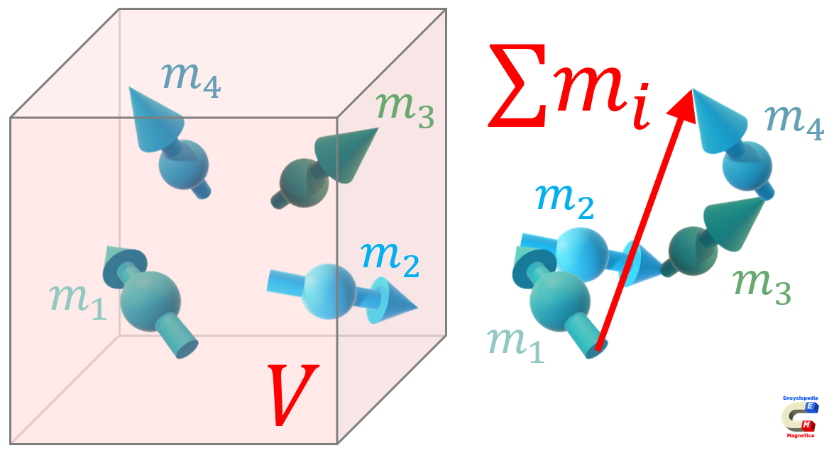
Magnetisation M (A/m) and polarisation J (T) represent an averaged quantity, “smoothed” over distances spanning across many individual magnetic moments.5)6)7)
| $$ \vec{M} = \frac{\sum \vec{m_i}}{V} $$ | (A/m) |
| $$\vec{J} = μ_0 · \vec{M} = μ_0 · \frac{\sum \vec{m_i}}{V} $$ | (T) ≡ (H/m)·(A/m) |
| where: $M$ - magnetisation (A/m), $\sum m_i$ - sum of magnetic moments of individual atoms (A·m2), $V$ - unit volume (m3), $μ_0$ - permeability of vacuum | |
Magnetic field is a vector field in space, and is a type of energy whose full quantification requires the knowledge of the vector fields of both magnetic field strength $H$ and flux density $B$, or other values correlated with them, such as polarisation $J$ (or magnetisation $M$). In vacuum, regardless of excitation, always $J$ = 0, and at each point the $H$ and $B$ vectors are oriented along the same direction and are directly proportional through permeability of free space, but in other media they can be misaligned (especially in highly anisotropic materials).
From engineering viewpoint, magnetic field strength $H$ can be thought of as excitation, and the magnetic flux density $B$ as the response of the magnetised medium. The quantity $B$ encompasses all of the magnetic response of the medium (including $J$ or $M$, as well as any other contribution arising from the applied $H$).8)
The four vector quantities (H, B, M, J) are interlinked such that:9)10)11)
| (typical vector notation) | $$\vec{B} = \vec{J} + μ_0 · \vec{H} = μ_0 · (\vec{H} + \vec{M}) $$ | (T) |
| (typical scalar notation) | $$B = μ_r · μ_0 · H = μ · H $$ | (T) |
| where: $μ_0$ - absolute permeability of vacuum (H/m), $μ_r$ - relative permeability of material (unitless), $μ = μ_0 · μ_r$ - absolute permeability of material (H/m), $J$ - magnetic polarisation (T), $M$ - magnetisation (A/m), $B$ - magnetic flux density (T), $H$ - magnetic field strength (A/m) | ||
Expressing the equation with magnetisation M is known as the Sommerfeld convention, and with polarisation J as the Kennelly convention. These are mathematically equivalent, and can be used depending on the easy of application in a given magnetic problem.12) However, attention must be paid to the physical units in other calculations such as torque due to magnetic moment.13) It is recommended to always follow equations which return correct units from the viewpoint of the SI system of units.
There are many other names which are used in the literature, but refer to the same physical quantity:
- magnetic polarisation J 14)
- polarisation J 15)
- magnetic polarisation I 16)
- intrinsic flux density Bi 17)
- intrinsic induction Bi 18)
- intrinsic induction J 19)
- J-field 20)
- ferric induction Bi 21)
- ferritic induction (B-H) 22)
- intensity of magnetisation I 23)
- magnetisation I 24)
- intrinsic magnetization J 25)
- and probably several more.
| → → → Helpful page? Support us! → → → | PayPal | ← ← ← Help us with just $0.10 per month? Come on…  ← ← ← |
Units of J
Magnetic dipole moment is defined as the product of the current (measured in amperes) flowing in the loop and the area of the loop (measured in square metres), so the resulting unit is (A·m2). Subatomic particles such as electrons exhibit intrinsic moments due to spin and orbital movement.

S. Zurek, E-Magnetica.pl, CC-BY-4.0
The vector sum of many such dipoles over some volume is therefore (A·m2 / m3) ≡ (A/m), so the unit for M is the same as for magnetic field strength H.
In some publications M is expressed in tesla or gauss26), which are the same units as for magnetic flux density B or magnetic polarisation J. This is simply because the values are scaled by the permeability of vacuum μ0 which itself has the units of H/m.27)
Therefore, the resulting unit of polarisation is J = M·μ0 (A/m)·(H/m) ≡ (T), the same as for magnetic flux density B.
The scaling of M (or H) by μ0 is not always explicitly stated or explained in the publications, but if the units are (T) then the scaling must have been applied, for the SI units to match. Therefore, whenever M is specified in the units of (T) then the quantity is effectively equal to J.
Similar logic applies to the CGS units, if M is compared to B. In the CGS nomenclature the polarisation J is typically referred to as “intrinsic flux density” or “intrinsic induction” Bi. However, there is an additional factor of 4·π which is required in the CGS system. Therefore, the volume magnetic susceptibility calculated in the CGS system differs by the 4·π from susceptibility in the SI system.28)
Magnetic polarisation in matter
Magnetisation M and hence also polarisation J are linked to the definition of volume magnetic susceptibility χvol, such that:29)30)
| $$ \vec{M} = χ_{vol} · \vec{H} $$ | (unitless) |
The value of relative permeability μr can be used, such that μr = χvol + 1.
Vacuum

S. Zurek, E-Magnetica.pl, CC-BY-4.0
In the assumed ideal vacuum there is no matter of any kind (the illustration shows an “empty box” with volume V).
Therefore, there are no particles, atoms or molecules which could contribute some magnetic moments (intrinsic or induced), so their sum is zero over any volume, regardless the level of magnetic excitation,31) hence it is always Mvacuum = 0 A/m.
Magnetic polarisation J is M scaled by permeability of vacuum μ0, therefore also always Jvacuum = 0 T.
Magnetic susceptibility of vacuum is precisely zero, and relative permeability is precisely unity.
In vacuum, magnetic field strength H and magnetic flux density B are equivalent, proportional to each other by the magnetic constant μ0.
| in vacuum | |
| $$\vec{B} = μ_0 · \vec{H} $$ | (T) |
| $J = 0 $, $M = 0$ | |
| $χ_{vol} ≡ 0$ | |
| $μ_r ≡ 1$ | |
Thus, B and H vectors are parallel, and in case of periodic excitation (e.g. such as in alternating or rotating process of magnetisation) there is no lead/lag between the vectors, owing to the fact that vacuum is a lossless medium.
Diamagnetic

S. Zurek, E-Magnetica.pl, CC-BY-4.0
In diamagnetic materials, the intrinsic magnetic moments of electrons in each atom cancel out, for example because of the even number of electrons which are paired such that on each orbital there are two electrons, with opposing spins.32)
Therefore, without any magnetic field applied from the outside, the material remains non-magnetised, because of sum of magnetic moments over some unit volume is still zero.
However, from a classical physics viewpoint, electrons orbiting in atoms can be treated as loops of superconducting current.33). Application of any external magnetic field changes trajectory of each orbit, equivalent to inducing a current in it. The direction is such that the magnetic field associated with it opposes the external field (due to Lenz's law).
The effect per atom equates to a small magnetic moment, and their sum adds up vectorially to a non-zero magnetisation M or polarisation J over the given volume, such that the induced net moment always opposes the direction of of the applied magnetic field B. Therefore, susceptibility of diamagnets is negative and relative permeability is less than unity.34)35) The effects are linear and do not depend on temperature in a significant way.
| in diamagnets |
| $χ_{vol} < 0$ |
| $μ_r < 1$ |
The effect is quite weak, but it happens for all atoms, also in other types of materials such as paramagnetic or even ferromagnetic, it is simply masked by the stronger effects of para- and ferromagnets (described below).
Any change of the applied magnetic field changes the induced magnetic moment. And therefore removal of the field un-induces precisely the amount of current which was initially induced, so that in zero applied field the value of M, J and therefore also B returns to zero as well.
For most engineering applications diamagnets are treated simply as “non-magnetic” (similar to vacuum). For example, copper has the relative permeability of 0.999994 (compared to vacuum's 1.000000).
Paramagnetic

S. Zurek, E-Magnetica.pl, CC-BY-4.0
In paramagnetic materials, there are atoms with at least one unpaired electron with the contribution of its intrinsic magnetic moment (spin and orbital).
Because of thermal agitation, the individual magnetic moments point in random directions, so that without any applied external field there is no net magnetisation or polarisation (M = 0, J = 0).36)
When some magnetic field is applied, the individual magnetic moments begin to align to it, producing some net vector sum of M or J, in the same direction as the applied field.
For paramagnets susceptibility is positive, but also weak, yet stronger than the co-existing diamagnetic effect, so that the paramagnetic contribution dominates.
| in paramagnets |
| $χ_{vol} > 0$ |
| $μ_r > 1$ |
At a constant temperature, the effects are linear with respect to the applied magnetic excitation. However, at lower temperature it is easier for the moments to align with the applied field and the susceptibility increases, and can even diverge for the material to become ferromagnetic or antiferromagnetic.37)
After removal of magnetic excitation, all the individual moments return to the normal thermally-agitated state and there is no retained magnetisation (M = 0, J = 0).
For most engineering applications paramagnets are treated simply as “non-magnetic” (similar to vacuum). For example, aluminium has the relative permeability of 1.000022 (compared to vacuum's 1.000000).
Ferromagnetic and other highly-ordered structures

S. Zurek, E-Magnetica.pl, CC-BY-4.0
If the interactions between the individual moments become strong enough, they can align spontaneously so that very long-range ordering occurs between many individual atoms, forming macroscopic structures called magnetic domains, in some materials extending even over tens of millimetres. Such phenomenon is called ferromagnetism.38)39)

In ferromagnetic materials, all the moments in a given domain are fully aligned, so that they are locally magnetically saturated (therefore locally M = Msat or J = Jsat). The domains are separated by domain walls, and the neighbouring domains can point in other directions (such as 180° or 90°), so that the net magnetisation of the whole material can be zero, even though each domain is saturated.
The domain walls can move and if some external magnetic field is applied the domains with directions similar to the field will grow at the expense of other - this is the process of magnetisation (which involves all the fundamental quantities: J or M, H and B). Large movements of magnetic domains are lossy (e.g. due to domain wall pinning) and thus irreversible, making the process history-dependent. The effects are non-linear, and under alternating excitation result with a hysteresis loop, when plotting the instantaneous values of J or M versus H (also B vs. H). The area of such loop is proportional the the total magnetic losses occurring in the material.40)

S. Zurek, E-Magnetica.pl, CC-BY-4.0
The interactions between the individual magnetic moments are affected by the distance between the atoms, and these are dictated for example by the crystal structure of the material. Most crystals have some privileged directions, along which the spacing between the atoms is smaller and the alignment of moments is easier because of the minimisation of energy. This effect is called anisotropy and can “anchor” the vector of magnetisation J at a direction different from the applied field. If this happens then all the vectors of H, J (or M) and B can point in different directions even under DC excitation, as illustrated schematically. Additional energy is required to overcome the anisotropy energy, and higher excitation needs to be applied to change the angular position of the J vector.
The spontaneous alignment of moments acts against the thermal agitation, and increased temperature weakens the magnetic ordering. At sufficiently high temperature (Curie temperature) the magnetic alignment can no longer be sustained, and the material becomes paramagnetic. This is the case for all ferromagnetic and other ordered structures (described below).
Depending on the definition, the value of susceptibility can diverge to infinity (because of the way it is defined mathematically), and therefore especially in engineering a more useful figure of merit is the permeability.41) Materials which are easy to magnetise (and demagnetise) are called soft magnetic materials and their relative permeability can reach very high values, even exceeding 1 000 000, as compared to non-magnetic materials which is 1.
| in ferromagnets |
| $χ_{vol} >> 0$ |
| $μ_r >> 1$ |
However, the internal structure of permanent magnets is designed to have the energy storage capability maximised, by increasing the value of coercivity. The magnets with the highest energy capability have the permeability also very close to unity, e.g. 1.05, even though they are ferromagnetic.42)

S. Zurek, E-Magnetica.pl, CC-BY-4.0
In a magnet, even if the actual magnetisation is uniform, in an open magnetic circuit the distribution of magnetic flux through the magnet and the surrounding medium leads still to non-uniform flux density B. Some demagnetising field Hd arises and points in the direction opposite to J. Therefore, the value of B is lower that if the demagnetising effect was not present.44)
The value of the unitless demagnetising coefficient Nd (contributing to the demagnetising field) is linked to the shape and dimensions of the magnetised body. For closed magnetic circuit Nd = 0 (no demagnetising field).
But for infinitely large thin sheet magnetised perpendicularly to its surface Nd = 1, and the resulting B is the same as if the material had permeability equal to vacuum (regardless of the actual value). Such shape anisotropy will favour for J to be aligned within the plane of such thin sheet.45)
Ferrimagnetic
In ferrimagnetic materials, there are two interleaved crystal lattices, each aligned magnetically in opposing directions. The resultant polarisation is therefore lower, but still the material behaves macroscopically as a ferromagnet, including having magnetic domains, exhibiting hysteresis loop and high permeability.
| in ferrimagnets |
| $χ_{vol} >> 0$ |
| $μ_r >> 1$ |
At sufficiently high temperature (Néel temperature) ferrimagnets also become paramagnetic.
Other magnetic structures
There are several types of magnetic ordering, which also result with strong interactions and ferromagnetic-like macroscopic behaviour. They differ mostly by the way the alignment of the individual moments follows some rules slightly different from classical ferromagnetism. They are known as types of magnetisms, and for example in the helical ferromagnetism the alignment of spins follows a helical order.46) Practical applications of such materials is limited.47)
Under sufficiently high temperature all these materials transition to paramagnets.
Antiferromagnetic
Antiferromagnetic materials have the internal structure similar to ferrimagnets, but the two interleaved lattices have almost the same contributions so they almost perfectly cancel one another, such that the material is macroscopically indistinguishable from a paramagnet (“non-magnetic”).48)
| in antiferromagnets |
| $χ_{vol} > 0$ |
| $μ_r > 1$ |
However, antiferromagnets are magnetically highly ordered structures, linked to the phenomenon of ferromagnetism. This is evident for example from Bethe-Slater curve, in which the type of interaction is plotted versus interatomic spacing. Closely packed structure can be ferromagnetic, with increasing distances could become antiferromagnetic, only for even larger distances to default to paramagnetic. Similar changes can be induced by temperature in some elements, as for example in thulium.
Some antiferromagnets can even form magnetic domains.49) Above Néel temperature antiferromagnets become paramagnetic.
Antiferromagnets are used in special types of magnetic sensors such as spin valves.50)
Superconducting

S. Zurek, E-Magnetica.pl, CC-BY-4.0
Superconductors do not exhibit magnetic ordering, and are therefore “non-magnetic”. Above the critical temperature, in a normal resistive state, superconductors can be paramagnetic or diamagnetic, with susceptibility close to zero and permeability close to unity.
However, when the temperature is lowered and the material enters the superconducting state, the magnetic field is expelled from the inside of the material (Meissner effect).
Additionally, any change of external magnetic field induces macroscopic superconducting currents $I_{sup}$ flowing on the surface. These currents are equivalent to magnetic moment and hence to magnetisation M or polarisation J associated with it. However, it is the macroscopic superconducting currents which sustain the response to the magnetic field, rather then the individual magnetic moments associated with each atom (see also the description of “bound” and “free” currents related to the analysis of magnetisation).
| in superconductor |
| $χ_{vol} = -1$ |
| $μ_r = 0$ |
The macroscopic magnetisation and hence also polarisation due to surface currents in superconductors always opposes the applied external magnetic field, such that it cancels it, with the effect of zero magnetic field penetrating to the inside of the superconductor. This is equivalent to the susceptibility being χ = -1 and relative permeability μr = 0, so that a superconductor can be referred to as an “ideal diamagnet”.51)52)
Saturation polarisation
| |
The magnetic response of all magnetic materials (ferromagnetic and similar) increases with the applied magnetic field, but eventually reaches magnetic saturation at sufficiently high amplitude.
Beyond a certain level of excitation the value of saturation polarisation Jsat is reached when all the internal magnetic moments are aligned (all domain walls disappear and there remains a single domain). Further increase of excitation does not cause for the J to increase any more, but the flux density B keeps increasing with the excitation H, as dictated by the equation:
| B due to H above saturation | ||
|---|---|---|
| (expressed with magnetisation M) | $B = μ_0 · (H + M_{sat})$ | (T) |
| (expressed with polarisation J) | $B = μ_0 · H + J_{sat}$ | (T) |
| where: $M_{sat}$ - saturation magnetisation (A/m), $J_{sat}$ - saturation polarisation (T) | ||
Therefore, there is no limiting value of “saturation flux density” Bsat or “saturation induction” even though some professional literature refers to such concepts.53)54) Nevertheless, in some cases it useful to use the concept of technical saturation defining some other point such as state of magnetic domains or value of permeability.55)56)
(The term “saturation flux density” in the CGS nomenclature is only correct with the implicit assumption that the name refers to the “intrinsic flux density”, which is equivalent to the magnetic polarisation J and hence also to the magnetisation M.)

S. Zurek, E-Magnetica.pl, CC-BY-4.0

S. Zurek, E-Magnetica.pl, CC-BY-4.0
Saturation polarisation is mostly dictated by the chemical composition and physical state of a given material.59)60) For anisotropic materials it does not depend on the direction of the applied field, but it might require larger amplitude to reach saturation in some directions.61)
Theoretically, it should be possible to saturate non-magnetic materials (such as paramagnetic and antiferromagnetic) by aligning all their magnetic moments. However, in practice this is extremely difficult to achieve, as it would require fields at the order of 80 MA/m or 1000 T.62)
Saturation polarisation vs. temperature

S. Zurek, E-Magnetica.pl, CC-BY-4.0
The value of saturation polarisation reduces with increasing temperature, and above the critical point of Curie temperature TC the ferromagnets (and other magnetic materials) become paramagnetic. The value of TC depends on the chemical composition of a given material.
At room temperature only three chemical elements are ferromagnetic: iron, cobalt and nickel, whereas for gadolinium TC = 20 °C, so it is paramagnetic.65) There are many alloys of Fe, Co and Ni comprising additional “non-magnetic” additions which remain ferromagnetic above room temperature. However, Heusler alloys can be ferromagnetic at room temperature even though they are made from non-magnetic elements, due to the complex interaction of the electron spins.66)
The value of spontaneous magnetic polarisation can be calculated from the Curie-Weiss law, by using the Brillouin equation which is a function of the exchange integral Je. From a practical viewpoint, the value of spontaneous polarisation at a given temperature represents the saturation limit at that temperature.
The classical physics approach ($J_e = ∞$) fails to accurately reflect the shape of the function. Ferromagnetism is linked to the quantum effects acting between the spin and orbital moments of the electrons. For Fe, Co and Ni the curves are close to 1/2 or 1 and $J_e = 1/2$ means that the exchange would be caused completely just by the spin moments.67)
Rare earth metals have unpaired electrons on different shells and therefore the exchange integral has a significantly different value.68)
| Curie temperature for ferromagnetic elements69) |
||
|---|---|---|
| (°C) | (K) | |
| cobalt Co | 1131 | 1404 |
| iron Fe | 770 | 1043 |
| nickel Ni | 358 | 631 |
| gadolinium Gd | 20 | 293 |
| terbium Tb | -54 | 219 |
| dysprosium Dy | -188 | 85 |
| thulium Tm | -241 | 32 |
| erbium Eb | -253.5 | 19.5 |
| holmium Ho | -254 | 19 |
Iron is inexpensive and has large saturation magnetisation, which is exploited in electrical steels used for large power transformers and generators in power plants. Although Co has lower saturation than Fe, the alloy 50Co-50Fe (known as Permendur) has the highest known saturation of 1.96 MA/m or 2.46 T.70)
| Magnetic saturation at room temperature71)72) | ||
|---|---|---|
| Saturation magnetisation Msat (MA/m) | Saturation polarisation Jsat (T) |
|
| iron Fe | 1.71 | 2.15 |
| cobalt Co | 1.42 | 1.78 |
| nickel Ni | 0.48 | 0.61 |
| 50Co-50Fe | 1.96 | 2.46 |
Measurement of magnetic polarisation J
Polarisation J can be measured by the same means as magnetisation M, which can be measured for example by detecting the magnetic dipole moment.
However, for samples of soft magnetic materials there are several ways in which the air flux compensation is used, as described below.
Via air flux compensation
Periodic excitation of a sample will induce a voltage in the coil wrapped around it. The voltage is proportional to the flux density B which comprises a vector sum of polarisation J and magnetic field strength H.

S. Zurek, E-Magnetica.pl, CC-BY-4.0
However, an additional winding can be installed and exposed to the same excitation field, but without the sample. This can be achieved for example by using a mutual inductor whose parameters are adjusted to the main magnetising and sensing windings. With correct settings, in such additional coil the induced voltage will not be affected by any value of J, but it will comprise the component proportional to H.
Such auxiliary secondary winding can be then connected in opposition to the winding on the sample, and therefore the H component will be compensated out, leaving only the voltage proportional to J (and hence also to M).
The air flux compensation method is used in the Epstein frames and single sheet testers for characterisation of soft magnetic materials such as electrical steels.73)