Table of Contents
Magnetic susceptibility
| Stan Zurek, Magnetic susceptibility, Encyclopedia Magnetica, https://e-magnetica.pl/doku.php/magnetic_susceptibility |
Magnetic susceptibility, denoted typically by χ (chi) or κ (kappa) - a quantity expressing the ratio of magnetisation M in a given material to the magnetic field strength H, also colloquially referred to as the ability of material to “concentrate” the magnetic field with respect to vacuum.1)

S. Zurek, E-Magnetica.pl, CC-BY-4.0
The basic definition refers to the volume magnetic susceptibility $χ_{vol}$:
| Volume magnetic susceptibility | |
|---|---|
| $$χ_\text{vol} = \frac{M}{H}$$ | (A/m) / (A/m) ≡ (unitless) |
| where: $M$ - volume magnetisation (A/m), $H$ - magnetic field strength (A/m) | |
In vacuum M is always zero regardless the level of applied H, hence χ ≡ 0.
For diamagnets susceptibility is weakly negative $χ < 0$, for paramagnets it is positive $χ > 0$.
For ferromagnets and ferrimagnets it is very large $χ \gg 0$, but also highly non-linear.
Superconductors expel magnetic field from their bodies and they are assumed to be “ideal diamagnets” hence $χ = -1$.
Magnetic susceptibility is widely used in theoretical physics and chemistry especially for analysis of non-magnetic materials, in which assumption of linear relationship between M and H holds quite well.
However, in electromagnetic engineering, the related concept of magnetic permeability is more useful for ferromagnets and ferrimagnets, for which susceptibility value can diverge to infinity at zero applied field (because of the mathematical definition and division by zero).3)4) In the SI system, the relative magnetic permeability $μ_r$ is related to the volume susceptibility $χ_\text{vol}$ such that: $μ_r ≡ χ_\text{vol} +1$.

S. Zurek, E-Magnetica.pl, CC-BY-4.0
| → → → Helpful page? Support us! → → → | PayPal | ← ← ← Help us with just $0.10 per month? Come on…  ← ← ← |
Relationship between susceptibility and permeability
The definition of relative magnetic permeability used widely in engineering is linked to magnetic susceptibility, which is more useful in theoretical physics, and in the SI system the relationship is such that:6)
| Relationship between permeability and susceptibility | |
|---|---|
| $$μ_r ≡ χ_\text{vol} + 1$$ | (unitless) |
| where: $χ_\text{vol}$ - volume magnetic susceptibility (unitless) | |
This relationship arises because: $B = μ_0·(H + M)$ and $M = χ·H$. Hence, $B = μ_0·(H + χ·H) = (1+χ)·μ_0·H $.
On the other hand, $ B = μ·H = μ_r·μ_0·H$, and therefore $μ_r = 1+ χ$.
In CGS, $μ =1 + 4π·χ$.7)
Types of susceptibility
Depending on the mathematical definition, there are several types of susceptibility. They all quantify the same underlying magnetic property, but have different numerical values and/or units, because the calculation is carried out per unit volume, per unit mass, per mole of matter, etc.8)
Confusion of units
This article focuses on SI units. However, In the CGS system of units the dimension for volume susceptibility is the same as in SI (also unitless), but the numerical value differs by a factor $4π$, so care must be taken when comparing and analysing the values.
This difference in the numerical factor is important, because the same physical units can be valid in both systems (e.g. unitless for volume susceptibility, or cm3/mole for molar susceptibility). The multiplicity of units and approaches causes errors even in reputable data sources.9) Therefore, the safest approach is to explicitly state if the given value is used in CGS or SI system, e.g. $χ^{CGS}$ or $χ^{SI}$.10)
A converter for the values between some SI and CGS units is provided below.
Since the question of the units of susceptibilities is often confusing, let us emphasize the point here. For the susceptibility χ, the definition is M=χH, where M is the magnetization (magnetic moment per unit of volume) and H is the magnetic field strength. This χ is dimensionless, but is expressed as emu/cm3. The dimension of emu is therefore cm3. The molar susceptibility χ, is obtained by multiplying with the molar volume, υ (in cm3/mol). So, the molar susceptibility leads to M = HχN/υ, or Mυ= χNH, where Mυ is now the magnetic moment per mol. The dimension of molar susceptibility is thus emu/mol or cm3/mol.
Further confusion is introduced by the fact that the symbol “$emu$” (from: electromagnetic unit)) widely used in some publications does not denote a proper physical unit, but rather it is an indication that the CGS units are used.12)13) The “emu” symbol could be even used instead of an actual unit.14)
This type of confusing notation is used both for the magnetisation M and for susceptibility, as listed in the table below.15)16) This leads to the possibility that the two quantities, magnetisation and susceptibility, could be expressed with the same “unit”.
| Multiplicity of CGS units used in some publications17)18) | |
|---|---|
| Magnetisation | Susceptibility |
| G, Oe, emu/g, μB/atom, μB/impurity, G·cm3/g, emu/cm3, emu | emu/g, emu/cm3, emu/mole, emu/(g·kOe), emu·At/(g·V), emu/(Oe·mole) |
If the proper SI units are used no confusion can arise, especially when re-calculating or converting the numerical values. It is unfortunate that some physicists continue to use the confusing CGS notation, and even some modern professional measurement equipment reports the values in “emu units”.19)
| |
Volume susceptibility
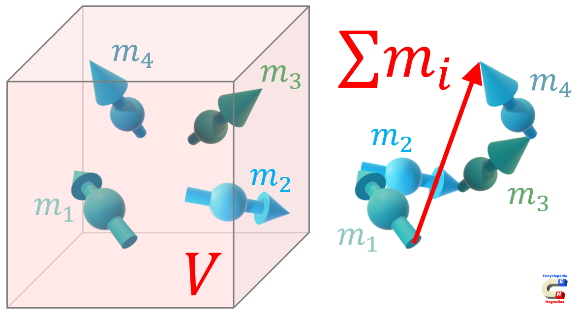
In theoretical physics, the (volume) magnetisation M is defined as the vector sum of magnetic dipole moments over unit volume:20)
S. Zurek, E-Magnetica.pl, CC-BY-4.0
| (volume) Magnetisation M | |
|---|---|
| $$M = \frac{\sum m_i}{V}$$ | (A·m2)/(m3) ≡ (A/m) |
| where: $m_i$ - individual magnetic moments (A·m2), $V$ - unit volume (m3) | |
Therefore, if such magnetisation per volume (also referred to as volume magnetisation) is taken for calculation of magnetic susceptibility then the volume magnetic susceptibility is obtained:21)
| Volume magnetic susceptibility χ | |
|---|---|
| $$χ_\text{vol} = \frac{M}{H}$$ | (A/m)/(A/m) ≡ (unitless) |
| where: $M$ - magnetisation (A/m), $H$ - magnetic field strength (A/m) | |
Mass susceptibility
If the volume susceptibility (described above) is divided by density of material, then the values are expressed per unit mass, thus obtaining mass magnetic susceptibility: 22)
| Mass magnetic susceptibility χ | |
|---|---|
| $$ χ_\text{mass} = \frac{χ_\text{vol}}{ρ} $$ | (m3/kg) |
| where: $χ_\text{vol}$ - volume magnetic susceptibility (unitless), $ρ$ - mass density of the material (kg/m3) | |
Molar susceptibility
Multiplying the mass susceptibility by a molar mass, one obtains the molar magnetic susceptibility:
| Molar magnetic susceptibility | |
|---|---|
| $$ χ_\text{mol} = χ_\text{mass}·m_\text{mol} = \frac{χ_\text{vol}·m_\text{mol}}{ρ} $$ | (m3/mol) |
| where: $χ_\text{vol}$ - volume magnetic susceptibility (unitless), $m_\text{mol}$ - molar mass (kg/mol), $ρ$ - mass density of the material (kg/m3) | |
Calculator of magnetic susceptibility
| |
Magnetic susceptibility can be calculated from magnetisation M and magnetic field strength H, with the SI units:
| Quantity | Equation | SI units | CGS units | Conversion factor F such that SI = F·CGS |
|---|---|---|---|---|
| Volume magnetic susceptibility $M$ - magnetisation (A/m) $H$ - magnetic field strength (A/m) | $$ χ_\text{vol} = \frac{M}{H} $$ | (unitless) ≡ (A/m)/(A/m) | (unitless) | $4π$ |
| Mass magnetic susceptibility $ρ$ - mass density (kg/m3) | $$ χ_\text{mass} = \frac{χ_\text{vol}}{ρ} $$ | (m3/kg) | (cm3/g) | $4π×10^{-3}$ |
| Molar magnetic susceptibility $ρ$ - mass density (kg/m3) $m_\text{mol}$ - molar mass (kg/mol) | $$ χ_\text{mol} = \frac{χ_\text{vol}·m_\text{mol}}{ρ} $$ | (m3/mol) | (cm3/mol) | $4π×10^{-6}$ |
Other types of susceptibility
| |
Depending on the requirements of the particular theory or scientific approach there can be many other types of susceptibility (atomic, ionic, etc.) Some of the differences are quite nuanced23) and they should be analysed carefully against the source of a given definition.
| Several types of magnetic susceptibility24) | |
|---|---|
| name | equation |
| reduced | $κ_{ab} = - ∂^2E/∂B_a ∂B_b$ |
| volume | $χ_{ab} = ∂M_a/∂H_b = μ_0 · ∂M_a/∂B_b = (μ_0/V) · κ_{ab} $ |
| mass | $χ_{ρ} = χ / ρ$ |
| molar | $χ_{mol} = χ_{ρ}·M_r = χ·M_r / ρ$ |
| mean | $\overline{χ} = M/H = μ_0 · M / B$ |
| averaged | $χ_{av} = (2·χ_⊥ + χ_{||})/ 3$ |
| differential | $\tilde{χ} = ∂M/∂H = μ_0 · ∂M / ∂B$ |
| isothermal | $χ_T = (∂M/∂H)_T$ |
| adiabatic | $χ_S = (∂M/∂H)_S$ |
| alternating current | $χ = χ' + i·χ'' $ |
| dispersion | $χ' = (M_0/H_0)·cos θ $ |
| absorption | $χ'' = (M_0/H_0)·sin θ $ |
| harmonic | $χ_n = χ_n' + i·χ_n'' $ |
| external | $χ_{ext} = dM/dH_a $ |
| internal | $χ_{int} = dM/dH = χ_{ext} / (1 - N·χ_{ext}) $ |
| TIP | $χ_{TIP} = lim_{T→0} (χ - χ_{dia}) $ |
| where all the symbols are as defined in the reference 25) | |
DC and AC susceptibility
Unless otherwise stated, most publications and material tables specify the “DC susceptibility”. The values are measured under applied DC magnetic field, after a “steady-state” was reached.
However, under alternating excitation with a frequency $f$ (and $ω=2·π·f$), there can be a phase difference between the excitation H and the response M of the material, due to relaxation effects. Such AC susceptibility $χ(ω)$ can be represented by a complex notation:26)

S. Zurek, E-Magnetica.pl, CC-BY-4.0
| AC susceptibility |
|---|
| $$ χ(ω) = χ'(ω) + i·χ''(ω) $$ |
| where: $χ(ω)$ - AC susceptibility, $χ'(ω)$ - real part or dispersion susceptibility, $χ''(ω)$ - imaginary part or absorption susceptibility |
The effect of the frequency $ω$ on AC susceptibility is directly related to the relaxation time constant $τ$. At low excitation frequencies the measured AC susceptibility is similar to the static or DC susceptibility. At that limit the spins remain with thermal equilibrium with the ambient and therefore the measured value of the in-phase component $χ'$ is also called isothermal susceptibility $χ_T$.
At the limit of high frequency, the spins do not have enough time to align with the field, and the value is called adiabatic susceptibility $χ_S$, which strongly depends on the amplitude of the applied field, and at strong fields $χ_S$ tends to zero.27)
The out-of-phase component $χ''$ tends to zero at both ends of the frequency range, but it exhibits a maximum at $ω=1/τ$.
The relationship between the four values is as follows:28)
| dispersion | $$ χ'(ω) = \frac{χ_T-χ_S}{1+ω^2 · τ^2} + χ_S $$ |
| absorption | $$ χ''(ω) = \frac{ω·τ·(χ_T-χ_S)}{1+ω^2 · τ^2} $$ |
| AC | $$χ(ω) = χ'(ω) + χ''(ω)$$ $$ χ(ω) = \left( \frac{χ_T-χ_S}{1+ω^2 · τ^2} + χ_S \right) + i·\left( \frac{ω·τ·(χ_T-χ_S)}{1+ω^2 · τ^2} \right) $$ |
Scalars and tensors
In analysis of many materials the approximation of isotropic properties is sufficient. Under such conditions the vectors of M and H are co-linear, and therefore the proportionality can be expressed with scalar susceptibility, such that:29)
| Scalar susceptibility |
|---|
| $$ \vec{M} = χ · \vec{H} $$ |
| $\vec{M}$ - vector of magnetisation, $χ$ - scalar susceptibility, $\vec{H}$ - vector magnetic field strength |
In a general case, susceptibility can be expressed with an operator which is linear, non-linear, or even such that includes hystereis.30)
In a linear case, especially for crystalline materials, there can be anisotropy of magnetic properties and the vectors of H and M may not be parallel to each other anymore, even though there is a linear relationship between the amplitudes. In order to represent such transformation in a more accurate way a set of linear equation can be used (for coordinates $1,2,3$), which can be also written also in a compact notation with tensor susceptibility (with coordinates $i,j$):31)32)33)
- a) sphere ($k_1=k_2=k_3$)
- b) oblate ellipsoid ($k_1 < k_2 ≈ k_3$)
- c) prolate ellipsoid ($k_1 > k_2 ≈ k_3$)
- d) triaxial ellipsoid ($k_1 \neq k_2 \neq k_3$)

S. Zurek, E-Magnetica.pl, CC-BY-4.0
| Tensor susceptibility | |
|---|---|
| (full notation) | $ M_1 = χ_{11} · H_1 + χ_{12} · H_2 + χ_{13} · H_3 $ $ M_2 = χ_{21} · H_1 + χ_{22} · H_2 + χ_{23} · H_3 $ $ M_3 = χ_{31} · H_1 + χ_{32} · H_2 + χ_{33} · H_3 $ |
| (compact notation) | $$M_i = χ_{ij} · H_j$$ |
| where: $M_i$ - i th component of $\vec{M}$ (A/m), $χ_{ij}$ - tensor susceptibility components (unitless), $H_j$ - j th component of $\vec{H}$ (A/m) | |
Such second-order tensor susceptibility can be visualised in a simplified way with a magnitude ellipsoid, which represents the anisotropy of susceptibility.
For such tensor, even though there are 9 terms in the equations, only 6 of them are independent, because of the symmetry $χ_{ij} = χ_{ji}$. It is also possible to further simplify the tensor notation with the eigenvalues such (by finding an appropriately aligned coordinate system), so only the diagonal values are non-zero, such that only the principal susceptibility components are present:35)36)
| Diagonal susceptibility |
|---|
| $ χ_p = \begin{bmatrix} χ_1 & 0 & 0 \\ 0 & χ_2 & 0 \\ 0 & 0 & χ_3 \end{bmatrix} $ |
and therefore the full equations simplify to:37)
| $ M_1 = χ_{1} · H_1 $ $ M_2 = χ_{2} · H_2 $ $ M_3 = χ_{3} · H_3 $ |
Susceptibility in materials
The susceptibility values are driven by the behaviour of magnetic dipole moments inside the matter. Electrons exhibit magnetic moments from the intrinsic spin and orbital contributions.
Other sub-atomic particles such as protons and neutrons also exhibit magnetic moments, but they are much smaller and do not contribute significantly to the macroscopic property of the matter. Therefore, these can be typically neglected in most engineering applications.
Vacuum

In pure vacuum there is no matter of any kind, so there are no magnetic moments, which could give rise to the magnetisation M.
Hence, under all conditions, regardless of the magnitude of magnetic field present, in vacuum always M = 0, and also the polarisation J = 0.
Therefore, the quotient M/H = 0 at all times, and susceptibility of vacuum is always zero, $χ≡0$, and relative permeability of vacuum is always $μ_r ≡ 1$.
This applies for any kind of susceptibility: volume, mass, molar, per atom, etc.
Diamagnets
In diamagnets there are atoms, typically with fully occupied orbitals, so that the electrons are paired, with opposing spins.

Because of such anti-pairing, the magnetic moments of the electrons completely cancel out and there is no contribution to the macroscopic magnetic properties.
However, from a classical physics viewpoint, each orbiting electron effectively constitutes a loop of superconducting current. When external magnetic field is applied, some equivalent current is induced in such loop. Because of the Lentz's law, the direction of the induced current is such that it opposes the applied field. Thus, the total field is somewhat lower, as compared to the case with vacuum and the same applied field.

Such induced orbital currents can be also quantified by some associated magnetic moments, and therefore some magnetisation per volume can be measured or calculated. Because the magnetic field is lowered by the diamagnetic interaction, the induced magnetisation opposes the applied magnetic field, and therefore susceptibility is close to zero but negative:39) $0 ≈ χ_\text{dia} < 0$.
This effect occurs in all ordinary matter, but it is very weak, and it is masked by the stronger paramagnetic and ferromagnetic interactions.
Diamagnetic susceptibility does not depend on temperature of the material in a significant way, and can be calculated by using a classical physics approach, by estimating the current induced in the orbiting electrons.40) In such Langevin model the value calculated for example for carbon is χ = -18.85 × 10⁻⁶, but the experimentally measured value is χ = -13.82 × 10⁻⁶, so the agreement of such analytical model holds only to the order of magnitude.41)
| Susceptibility in diamagnets (from classical calculations)42) | |
|---|---|
| $$ χ = - \frac{N·{μ_0}^2·e^2·Z}{6·m_e}·\overline{a^2} $$ | (unitless) |
| where: $N$ - number of atoms per unit volume (1/m3), $μ_0$ - permeability of vacuum (H/m), $e$ - elementary charge (C) of an electron, $Z$ - number (unitless) of orbital electrons in the atom, $m_e$ - mass of electron (kg), $\overline{a^2}$ - average (m2) of the square of spherical electron orbit radius $a$ (m) | |
Typical values of diamagnetic susceptibilities lie between zero and -100 × 10-6, with a few exceptions such as bismuth and graphite which exhibit larger values.43)44)
Superconductors
Superconductors are referred to as “ideal diamagnets” because they expel magnetic field from their inside. The effect is not caused by atomic effects, but rather by macroscopic currents flowing on the surface.45) Nevertheless, this effect can be also quantified by means of macroscopic volume magnetisation.

The macroscopic superconducting surface currents are such that they completely balance out the applied field H, so that inside the superconductor the total magnetic field B is zero, which from the analysis of the equations leads to $χ = -1$.
| Diamagnetic susceptibility in superconductors46) |
|---|
| $$ B = μ_0 · (M + H) = 0$$ $$M + H = 0$$ $$H = -M$$ $$χ=\frac{M}{H} = -1$$ |
This diamagnetic effect in superconductors is strong enough that levitation can be achieved between a strong permanent magnet and a superconducting body.
Internally, the superconductors can be made of a diamagnetic or paramagnetic material, but since there is no magnetic field inside the superconductor (Hin = 0) then only the surface currents matter from the viewpoint of macroscopic susceptibility.
Paramagnets
In paramagnets, there are unpaired electrons in the atoms, which contribute their magnetic moments.

The atoms undergo thermal agitation which tends to distribute the orientation of the moments in a random way, so without any applied field the net magnetisation is zero.
When some magnetic field is applied then there is some small deviation in the orientation of each moment such that a net alignment is produced, when summed over all contributions. This alignment is in the direction of the applied field so the average macroscopic field is somewhat greater than the applied one, even though the effect is also rather weak.
Hence, the susceptibility in paramagnets is also close to zero, but slightly positive:47) $0 ≈ χ_\text{para} > 0$.

In paramagnets the susceptibility typically depends on the temperature in a reciprocal relationship, as described by the Curie law or the more general Curie-Weiss law.49)
Because of the reciprocal proportionality, often the function is plotted not as $χ=f(T)$ but as $1/χ=f(T)$ which for paramagnets produces a straight line.
| Paramagnetic susceptibility (Curie law)50) | |
|---|---|
| $$χ = \frac{C}{T}$$ | (unitless) |
| where: $C$ - material constant (K), $T$ - absolute temperature (K) | |
Some materials such as antiferromagnets have a more complex structure of magnetic moments, but from a macroscopic view point behave similar to paramagnets, with similar values of macroscopic magnetic susceptibility.
Ferromagnets and ferrimagnets

If the interactions between the individual moments become strong enough, they can align spontaneously so that very long-range ordering occurs between many individual atoms, forming macroscopic structures called magnetic domains, in some materials extending even over tens of millimetres. Such phenomenon is called ferromagnetism.51)
Therefore, even without external magnetic field (H = 0) such material is magnetically saturated locally, so that M = Msat.
The spontaneous alignment of magnetic moments can happen because for some conditions the magnetic interactions are stronger than the thermal agitation. Therefore, the magnetic ordering increases at lower temperatures, and some materials which are paramagnetic at room temperature (such as gadolinium) can become ferromagnetic at lower temperatures.
The critical transition point between paramagnetic and ferromagnetic state is called the Curie temperature $T_C$. All ferromagnets become paramagnetic at sufficiently high temperatures, and revert back to ferromagnetic when the temperature is lowered (and if no other severe chemical changes took place such as oxidisation). The change is not instantaneous, but the ferromagnetic properties weaken when the Curie temperature is approached.
Some of these effects are described by the Curie-Weiss law, which is a more general version of the Curie law. Above the Curie temperature, the inverse permeability follows a straight line, similarly as for ordinary paramagnets (because they are in fact paramagnetic in that range).

| Ferromagnetic susceptibility (Curie-Weiss law)53) | |
|---|---|
| $$χ = \frac{C}{T-Θ}$$ | (unitless) |
| where: $C$ - material constant (K), $T$ - absolute temperature (K), $Θ$ - Curie-Weiss material constant (K) | |
Above Curie temperature, magnetic susceptibility of ferromagnets is still typically much higher than other materials. Upon cooling, the ferromagnetic state emerges and susceptibility increases to very large values (or infinity, depending on definition) when the material becomes ferromagnetic. In the ferromagnetic state it is more useful to use permeability, and in the tables of magnetic susceptibility the values can be even replaced simply with the word “ferro”.54)
Ferrimagnets
In ferrimagnets, there are two sublattices with opposing magnetic moments, but such that the contribution of one sublattice is greater and therefore they behave macroscopically similarly to ferromagnets.

At sufficiently high temperature the ferrimagnets also become paramagnetic, with the susceptibility values falling to correspondingly low values. However, the transition through the Curie temperature is different than in ferromagnets, because of the interaction between the two sublattices. Below the Curie temperature the susceptibility also diverges to infinity, as in ferromagnets.
The Curie-Weiss law can be also used to describe the ferrimagnetic behaviour, but more terms are required in order to represent the increased complexity of the curve.56) With increased temperature the $1/χ$ curve approaches as straight line asymptote, as it would be for ordinary paramagnets.
Antiferromagnets
In antiferromagnets there are also two interacting sublattices, in some sense similar as in ferrimagnets. However, the magnetic moments in each sublattice cancel each other so that the material exhibits macroscopic paramagnetic behaviour, with similar susceptibility values.
Antiferromagnetic state is a magnetically ordered structure, which can be destroyed by thermal agitation. Above a critical point called Néel temperature $T_N$ (an equivalent of Curie temperature for ferromagnets) the material transitions to a paramagnetic state, with the inverse of susceptibility becoming linear, as dictated by the Curie-Weiss law.

However, below the Néel temperature the values of susceptibility also remain as low as of other paramagnets. The cancellation of magnetic interaction of the sublattices is closely matched such that macroscopic measurements are insufficient for identification of the magnetic state and more sophisticated methods are needed, such as neutron diffraction measurements.58)
Measurement of susceptibility
There are several different methods for measuring magnetic susceptibility. Some of them share the similarity of relying on the measurement of mechanical force or values related to it, for example: Gouy, Curie or Quincke method. They are typically suitable for measurements of only DC properties.
Susceptibility can also be measured by detecting magnetisation of a body, but very high sensitivity is required for feebly magnetic materials, which can be difficult for small samples: vibrating sample or induced magnetisation method, as briefly described below.
Through force

For example, in the Gouy method the sample has a shape of long rod, whose one end is placed in the uniform field of large magnitude, in the air gap of a magnetic circuit (such as electromagnet), and the other end extends away, to much weaker field.
The magnetic field gradient acts on the magnetisation M of the sample (equivalent to magnetic dipole moment per unit volume), and hence generates magnetic force proportional to the product of the gradient of the field and the magnetisation of the sample. In materials in which magnetisation is proportional to the applied field the force acting on the sample is proportional to the susceptibility of the sample material.
The method can be used for measuring both polarities of susceptibility, because paramagnetic, antiferromagnetic, ferrimagnetic and ferromagnetic samples are attracted towards the high field, and the diamagnets are repelled from it. Relatively large volume is an advantage from the viewpoint of sensitivity, but it is disadvantage from the viewpoint of the amount of material needed for the measurement.
The samples can be solid (used directly), but also powder, liquid or gas - which require suspending in a suitable tube, whose susceptibility has to be subtracted accordingly.
During such measurements, the maximum field can be at the order of 800 kA/m, and the field at the other end of the sample 1% of this value, or 8 kA/m.60)
The knowledge of the exact gradient of the magnetic field is not required, and the the total force acting on the sample can be calculated by integrating over the volume of the whole sample, such that:
| $$ F_x = μ_0·A· \frac{χ-χ_0}{2}·\int_{Hy, low}^{Hy, max} d {H_y}^2 = μ_0·A· \frac{χ-χ_{0}}{2}·({H_{y, max}}^2-{H_{y, low}}^2) $$ | (N) |
| where: $F_x$ - force (N) acting along the axis of the rod, $μ_0$ - permeability of vacuum (A/m), $A$ - cross-sectional area (m2) of the rod sample, $χ$ - susceptibility (unitless) of the sample under test, $χ_0$ - susceptibility (unitless) of the displaced medium e.g. air, $H_{y, low}$ and $H_{y, high}$ - the low and maximum values of magnetic field strength (A/m) respectively, | |
which for $H_{y, max} >> H_{y, low} $ becomes
| $$ F_x ≈ μ_0·A· \frac{χ-χ_0}{2}·(H_{y, max})^2 $$ | (N) |
Moreover, if the sample susceptibility is significantly greater than that of air (or the given surrounding medium) namely $χ >> χ_0$ then the equation can be further simplified to:61)
| $$ F_x ≈ μ_0·A· \frac{χ}{2}·(H_{y, max})^2 $$ | (N) |
In the Curie method (also referred to as Faraday method), the overall concept is similar. However, the sample is smaller and the distribution of the applied magnetic field has to be designed to follow a specific function. The sample is then moved through all the positions from the low field to the maximum field, and the values of forces are integrated accordingly, along all the positions.
In the Quincke method, a U-shaped tube is used, with the sample being a liquid. One end of the tube is put in the high field and the acting forces makes the liquid level for example to rise for positive susceptibility because of the attractive force on the liquid. The amount of the level change is proportional to the value of susceptibility.
Through magnetic moment

The distribution of magnetic field around a magnetic dipole is independent of the shape or size of the body with the magnetic moment, when measured at a large distance (as compared to the dimensions of the analysed magnetic dipole).62) Therefore, a sufficiently small sample can be treated as a “point source dipole”.63)
The value of magnetisation M is an average of magnetic moment m per unit volume V:
| $$ M = \frac{m}{V} $$ | (A·m2/m3) ≡ (A/m) |
Therefore, assuming uniform magnetisation within the whole sample, scaling M by the volume or mass gives direct relation to the magnetic moment:
| (per volume V) | $$ M·V = \frac{m}{V}·V = m $$ | (A·m2) |
| (per mass w) | $$ M·w = \frac{m}{V}·w = m·D $$ | (A·m2·kg/m3) |
| where: $M$ - magnetisation of the sample (A/m), $m$ - magnetic moment (A·m2), $V$ - volume of the sample (m3), $w$ - mass of the sample (kg), $D$ - density of the sample (kg/m3) | ||
This proportionality can be employed for a measurement of M in small samples, by means of a vibrating-sample magnetometer64) (VSM) or vibrating-coil magnetometer. Both methods allow measuring the same quantity, but VSM is more robust and hence it is more widely used.65).
For example, in the VSM, the sample is attached to a rod, which is made to vibrate in a sinusoidal manner. DC magnetic field can be applied from an electromagnet. Because of the Faraday's law of induction, the DC field does not induce any voltage in the sensing coils. Each data point is measured with the static field from the electromagnet, so the measurement is not made during a change of the electromagnet field.
The magnetisation M in the sample generates a stray field. When the sample is vibrating the variations in the stray field induce voltage in the sensing coils.66) This voltage is directly proportional to the magnetic moment of the sample:67)
| $$ V_{coil} = 2 · π · f · C · m · a · sin (2·π·f·t) $$ | (V) |
| where: $f$ - frequency or vibration (Hz), $C$ - magnetic coupling constant (H/m3), $m$ - magnetic dipole moment of the sample (A·m2), $a$ - amplitude of vibration (m), $t$ - time (s) | |
However, the “point source” approximation can be assumed only for samples which are small in comparison to the sensing coils. For larger samples the measurement error increases even though the induced voltage also increases due to larger volume. In any case, the VSM needs to be calibrated by a sample of a known magnetic moment, for example made as a palladium cylinder or a nickel sphere.68)
Smaller samples produce less signal. The measurement is difficult because the signal is low even for larger samples, and therefore sophisticated signal processing is required to improve the signal-to-noise ratio of the apparatus. The sensing coils can be wound in a gradiometer configuration and the signals are filtered through lock-in amplifiers. The limit of resolution is dictated by the noise, and for high-precision scientific systems can be at the level of 10-6 emu or 10-9 A·m2,69) which for a sample 1 cm3 is equivalent to a resolution of 0.001 A/m. Smaller samples give lower resolution.
Commercial VSM devices can measure the magnetic moment in the SI units of A·m2 per mass or volume of the sample, but also in the unit of emu/g, which is equivalent to A·m2/kg. Therefore, to calculate magnetisation the volume and mass or density of the sample is required.70) Knowing M and the applied H it is possible to calculate the value of susceptibility.
The method is very sensitive and therefore measurements on very small samples can be affected by contamination of the sample holder. For example, even colouring agents in plastics can contain small amount of magnetic particles, or ordinary dust can contribute to magnetic contamination.71)
As an example of yet another method, the value of susceptibility can be measured by detecting the inductance of a coil, whose “core” is made of the sample under test. A difference in magnetic permeability in reference to an “air core” without the sample is used for the measurement. In this method, larger samples produce more accurate readings.72)